Mechanism Design
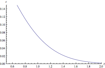
The regulator requires of each bank that it hold a certain amount of loss-absorbing capital. We call this function \(z\). Higher capital buffers have as a consequence lower chances of bank failure and therefore a lower systemic cost. But we can assume that some additional cost derives from the higher requirements themselves. (Certainly the banks themselves would argue so.) The regulator must decide how to balance systemic cost \(c\) with the mean \(\bar{z}\) of capital buffers system-wide. That is to say, it must select a point on the Pareto frontier.

What exactly does this plot show? Associated with each value of \(\bar{z}\) is a value for \(c\) which is, in some precise sense, the best achievable. There may be configurations of the banking sector and specifications of \(z\) that lead to a systemic cost \(c\) falling below this line. But we will not consider any configuration achievable if it consists of banks having widely different capital requirements. Such a configuration cannot be at equilibrium because it will be possible for a bank to adjust its holdings in order to find a lower capital requirement. That is to say, we assume that no one bank will suffer a capital requirement much in excess of any other's.
Our measure of systemic cost \(c\) follows closely the proposal of Beale et al.*
*Individual versus systemic risk and the Regulator's Dilemma, PNAS 108, pp.12647-12652, Aug 2011
There it is given by the expectation \[c=\sum_{k=1}^{n}c_{k}q_{k}\] with \(q_{k}\) the probability that exactly \(k\) out of \(n\) banks fail. The coefficient \(c_{k}\) is supposed to be some superadditive function of \(k\) so that, for example, it will be considered more than twice as bad for two banks to fail as it will for one. Specifically Beale et al. propose that, for some \(s>1\), it be given by \[c_{k}=k^{s}.\]
Here we proceed from the case \(s=2\), scale by fixing \(c_{n}\) to \(1\) (corresponding to the case of total system failure) and generalise by allowing some gradient \(1-a\) at the origin. Our cost function becomes \[c_{k}=\left(1-a\right)\frac{k}{n}+a\frac{k^{2}}{n^{2}}.\]
The values for \(q_{k}\) derive from a probability distribution over losses on assets \[V=\begin{pmatrix}v_{1}\\v_{2}\\\vdots\end{pmatrix}\] inducing a distribution on the fall in bank \(i\)'s valuation through the exposure matrix \[x_{i}=\begin{pmatrix}x_{i1}&x_{i2}&\cdots\end{pmatrix}\qquad\text{with}\qquad\sum_{l}x_{il}=1.\]
Bank \(i\) fails if its loss \(x_{i}V\) exceeds its capital buffer \(z_{i}\). Let \[\xi_{il}=\frac{x_{il}}{z_{i}}\] so that the probability of failure of bank \(i\) is \[\mu\left(\left\{\xi_{i}\right\}\right)=\text{Pr}\left(\xi_{i}V>1\right)\] and the probability of failure of both bank \(i\) and bank \(j\) is \[\mu\left(\left\{\xi_{i},\xi_{j}\right\}\right)=\text{Pr}\left(\xi_{i}V>1\text{ and }\xi_{j}V>1\right).\]
It is straightforward to show that \[c=\frac{1-a}{n}\sum_{i}\mu\left(\left\{\xi_{i}\right\}\right)+\frac{a}{n^{2}}\sum_{ij}\mu\left(\left\{\xi_{i},\xi_{j}\right\}\right)=\frac{1}{n}\sum_{i}\mu\left(\left\{\xi_{i}\right\}\right)-\frac{a}{2n^{2}}\sum_{ij}\nu\left(\left\{\xi_{i},\xi_{j}\right\}\right)\] where \[\nu\left(\left\{\xi_{i},\xi_{j}\right\}\right)=\mu\left(\left\{\xi_{i}\right\}\right)+\mu\left(\left\{\xi_{j}\right\}\right)-2\mu\left(\left\{\xi_{i},\xi_{j}\right\}\right).\]
Now let us suppose that the regulator has determined the relative importance of \(c\) and \(\bar{z}\) — it has selected a point on the Pareto frontier or, equivalently, it has specified a value for \(\lambda\) in the objective function \[\mathcal{L}=c+{\lambda}\bar{z}.\]
Then using that \[n\frac{\partial\mathcal{L}}{\partial\xi_{i\ell}}=\frac{\partial}{\partial\xi_{i\ell}}\mu\left(\left\{\xi_{i}\right\}\right)-\frac{a}{n}\sum_{j{\neq}i}\frac{\partial}{\partial\xi_{i\ell}}\nu\left(\left\{\xi_{i},\xi_{j}\right\}\right)-\frac{\lambda}{\left(\sum_{k}\xi_{ik}\right)^{2}}\] we may compute the optimal configuration for varying \(\lambda\).
PLOT GOES HERE.
But this plot shows the best possible out of all configurations, not just those that are achievable. To confine ourselves to these latter, it is easiest to pass to the infinite-size limit. In that case we can be assured that every bank will have exactly the same capital requirement . We introduce
and
, parametrised by the common capital requirement
and operating on normalised vectors
and
.
and
Then it is straightforward to describe a rule whose equilibrium minimises for some particular
,
where
and may be likened to the inverse of temperature, were we to consider a noisy version.
