
Sample path large deviations and concentration
We consider minimising the rate function
over the sets
These two cases are called the free boundary problem and Dirichlet boundary problem, respectively. is called the free energy for the pinning, and is treated as a constant throughout.
In the free boundary case, the set of minimisers is contained in the set , where
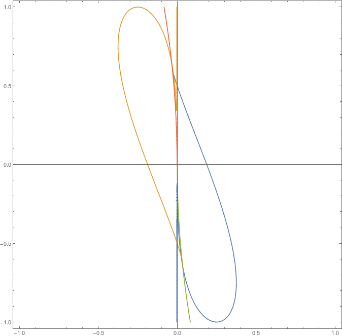
correspond to the green, orange and blue curves in the figure below, respectively.

We note that these minimisers only exist at the same time for some particular choices of . Using Euler-Lagrange, we can see the minimisers will be cubics. We overview the different cases and give a description of the cubics.
Firstly, we split our interval up in to two. Namely , where we take
to be some cubic, and
, where
is zero. For
, we have the unique minimiser
.
Secondly, by noting , we see that any minimiser must satisfy
. A simple calculation reveals that
We can then see suitable minima occur at the points
After substituting these values into and equating to zero, we reveal critical cases corresponding to multiple minimisers, in terms of
and
only. We may then plot this curve to see regions where one, two and three minimisers occur. This plot is shown below. Inside the sausage the region the minimiser succumbs to the pinning strength. Most interestingly, we will get multiple minimisers when parameters are such that they lie on the boundary of this region. The most peculiar situation of three minimisers happen at the two points where blue and yellow lines cross.
The same analysis can be conducted for the Dirichlet boundary case, albeit more messy. This gives us 5 potential minimisers and in principle, the regions in parameter space where minimisers change or multiple minimisers occur can be calculated.
For the case of wetting, we consider minimising the rate function
over the convex spaces
for the free and Dirichlet boundaries respectively.
This problem is in fact equivalent to the biharmonic obstacle problem
where the function space depends whether we work with a free boundary or Dirichlet boundary.
It is well known this problem has a unique solution. Furthermore, the obstacle problem has an equivalent strong formulation known as the free boundary problem, given by
where the fourth derivative is to be understood in the sense of distributions.
In our case, we note that on ,
is a biharmonic function, which in 1D simply means that it's a cubic outside of the coincidence set
.
In order to explicitly find a minimiser over we proceed as follows:
- Find conditions on boundary parameters for which
(introduced in the previous section) is naturally positive on
- call this set
. If
then there is nothing to do and
- If
, then assume there is some coincidence set
for
on which the minimiser is a constant zero function. Let us denote such function by
and note the following:
- on
we have a cubic, which necessarily satisfy
(as
has to be differentiable to be in the set);
- a potential minimiser would ideally like to coincide with the obstacle at
, as then it has "more time" to counter its willingness to go negative: a simple calculation reveals that
which, if treated as a function ofis non-increasing on
.
- in many cases for
- on
- in many cases for
is large enough the aforementioned cubic will itself go negative before reaching
Using this recipe, explicit minimisers that occur in the case of wetting can be found. For the Dirchlet boundary we proceed similarly adding a mirror argument for the right-hand boundary, where we now assume that the coincidence set is .