Gaussian Potential

A Gaussian potential has the form

\begin{equation}V(\eta) = \frac{c}{2}\eta^{2},\quad c > 0.\end{equation}

For this choice of potential the partition function \(\widehat Z_\lambda\) can be computed explicitly as a Gaussian integral

\[\widehat Z_\lambda = \int_{\mathbb R} e^{\lambda \eta - \frac{c}{2} \eta^2} d\eta = \sqrt{ \frac {2\pi}{c} } e^{\lambda^2/ 2c }.\]

Then by the definition of \(x(\lambda)\), taking logs and differentiating gives \(x(\lambda) = \lambda / c\); it follows that \(\lambda(x) = c x\) and hence

\begin{equation}f(x) = \frac{c}{2}x^2.\end{equation}

Superposition of Gaussian Potentials

A non-convex example for which our method may be used is:

\begin{equation}\exp \big( - V(\eta) \big) = p \exp \left( - \frac{\kappa_1}{2} \eta^2 \right) + (1-p) \exp \left( - \frac{\kappa_2}{2}\eta^2 \right).\end{equation}

Here \(\kappa_1, \kappa_2>0\) are stiffness parameters and it is generally assumed that \(\kappa_1 \gg \kappa_2\). The measure can be reformulated so that with probability \(p\) (respectively \(1-p\)) the distribution is conditioned to behave according to the density \(\exp( - \frac{\kappa_1}{2} \eta^2 )\) ( respectively \(\exp( - \frac{\kappa_2}{2} \eta^2 )\)).

Using the same Gaussian integral evaluation we used for the potential \(V(\eta) = \frac{c}{2}\eta^{2}\), we can compute the partition function \(\widehat Z_\lambda\) for the superposed Gaussian potential

\begin{equation}\hat {Z_{\lambda}} = p \sqrt{ \frac{2 \pi}{\kappa_1}} e^{\lambda^2 / 2 \kappa_1} + (1-p) \sqrt{ \frac{2 \pi}{\kappa_2}} e^{\lambda^2 / 2 \kappa_2}.\end{equation}

Again drawing comparison with the simple Gaussian potential, we identify \(x(\lambda)\)

\begin{equation}x(\lambda) = \left(\frac{\kappa_2a+\kappa_1b}{\kappa_1\kappa_2(a+b)}\right) \lambda\end{equation}

where \(a:= pe^{\frac{\lambda^{2}}{2\kappa_1}}\sqrt{\frac{2\pi}{\kappa_1}}\) and \(b:=(1-p) e^{\frac{\lambda^{2}}{2\kappa_2}}\sqrt{\frac{2\pi}{\kappa_2}}\), and we define

\[C(\lambda):=\left(\frac{\kappa_2a+\kappa_1b}{\kappa_1\kappa_2(a+b)}\right),\]

so that \(x(\lambda) = C(\lambda) \lambda\). If we choose the stiffness parameters so that \(\kappa_1, \kappa_2 > 1\) then \((\kappa_1 \kappa_2 )^{-1} < C(\lambda) < 1\); from this we obtain bounds on the free energy

\begin{equation} \frac{x^{2}}{2} < f(x) < \kappa_1\kappa_2\frac{x^{2}}{2}.\end{equation}

Similarly when \(\kappa_1, \kappa_2 < 1\) we have

\[\kappa_1\kappa_2\frac{x^{2}}{2} < f(x) < \frac{x^{2}}{2}.\]

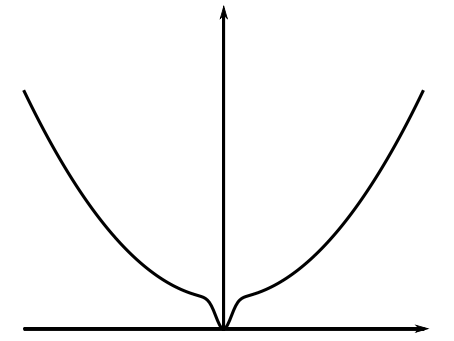
Whilst we have not been able to obtain a formula for \(f\), our method has enabled us to find bounds which show that of \(f\) is \(O(x)\).

Double Well Potential

As a final example we consider the double well potential

\begin{equation}V(\eta) := (\eta^{2}-1)^{2}.\end{equation}

Applying our main Lemma we note that the free energy exists and is strictly convex. Whilst we have not found an explicit formula for the free energy, the fact that it is strictly convex is interesting in itself, since one would not expect this of a potential that has two global energy minima.

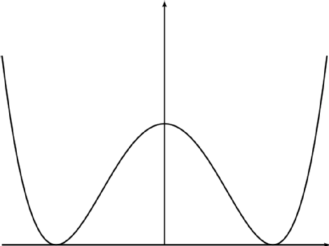
For such a potential one would expect to find two distinct equilibrium configurations, one of which favours \(+1\)-valued bonds, whilst the other has a majority of \(-1\)-valued bonds, in turn corresponding to the existence of two distinct Gibbs measures, and the occurrence of a phase transition. However, the strict convexity of the surface tension corresponds to a strict energy minimum of the system, which would appear to contradict this reasoning, and indicates (though does not prove) a lack of phase transition.

This somewhat counter intuitive situation is commonplace in \(1\)-dimension, and can be partially explained by comparison to other models. Noting that the potential \(V\) has energy minima at \(\pm 1\) and has ground states of pure \(+1\) and pure \(-1\) configurations, it is somewhat natural to relate it to the \(1\)-dimensional Ising model, which is known not to exhibit a phase transition even though the model does in higher dimensions.

A second comparison is to the random walk, with distribution described by the potential \(V\). In \(1\)-dimension, the random walk is known to fluctuate wildly, and hence is unlikely to remain in either of the states favoured by the distribution.

As a final justification, consider the case of zero tilt (purely for ease of understanding), \(x = 0\). The loop condition asserts that the mean value taken by a bond is \(0\), and since the double well concentrates mass around bonds taking \(\pm 1\) values, this is saying that we expect there to be equally as many \(+1\) bond as their are \(-1\). Taking the thermodynamic limit, one expects to preserve this balance between positive and negative bonds, which is to say that there is a unique limiting Gibbs measure in which we have phase coexistence, rather than the expected distinct Gibbs measures corresponding to the two possible phases.

Next Nearest Neighbour Interactions