
Numerical Results
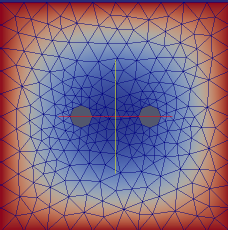
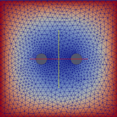
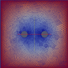
Our numerical computations use the finite element method, using DUNE software. Our domain for this problem is a square with circular inclusions, which we generate using MATLAB. An example of the constucted grid undergoing the refinement process is shown below.
Our program assembles a matrix equation which represents our discretised PDE. It takes the form
where and
are matrices assembled using the nodal basis functions. The nodal basis functions corresponding to
and
are based on the Morley and piecewise linear elements respectively. We then implement the boundary conditions row by row in the system matrix.
To test our numerical implementation is correct we use a convergence test that incorporates a predetermined solution into the right hand side. We take solutions for and
of the form
and take a domain of a circle of radius 1 with a smaller circle of radius 0.5 for the inclusion. Setting the boundary values that correspond to our choice for and
, we can compute the solution and compare it to our original values. We get the following plots.
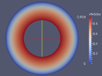
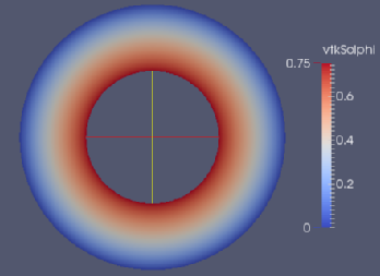
These plots correspond to the functions . To further test this we look at the convergence of the energy for an increasing number of refinements. This gives us the following graph.
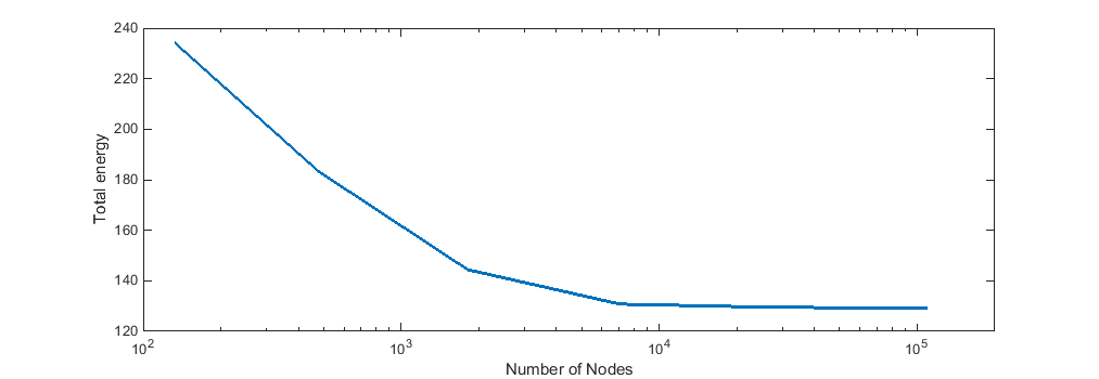
As we can see the energy stabilises to a specific value after enough grid refinements.
After verifying the convergence of the program, we were able to test varying parameters for our problem, such as the distance of the inclusions, the values of the coefficients and the boundary conditions. One example of a test showing the interaction between inclusions for varying distance is shown below.
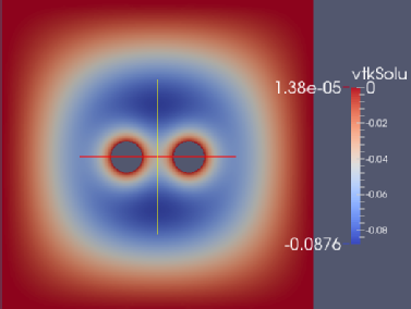
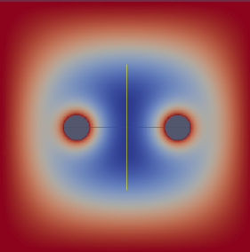
The above plot shows the value of for two different distances. We can additionally look at the energy of the system.
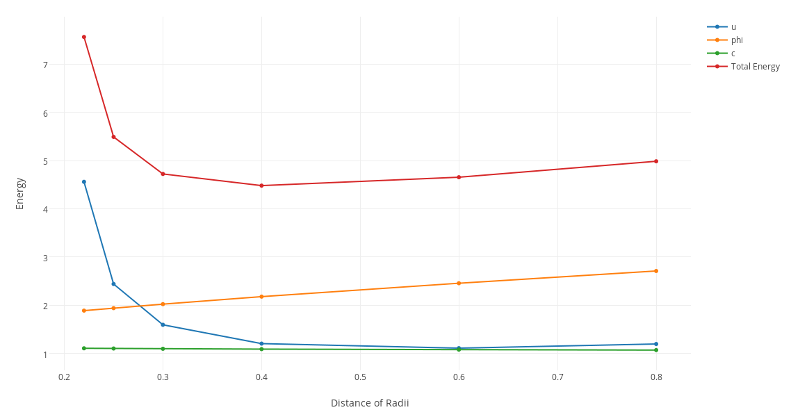 This graph is interesting since it seems to imply that there is an optimal distance that the inclusions want to take from each other to minimise the energy.