
Rail Inspection
Introduction
Ultrasonic inspection of rails is usually restricted to low speeds of around 20-30mph [1], which limits the viability of testing many tracks regularly. Higher speed inspection has been reported of up to 60mph, but no indication of the change in reliability is quoted for these speeds. Furthermore many of the most serious defects that can develop in the rail head can be very difficult to detect using the currently available inspection equipment such as the wheel probe shown in the schematic diagram below. The wheel probe is configured so that it generates either compression or shear waves in the rail, and one issue with surface defects is that a small defect can obscure the detection of a deeper defect, and as such defects often occur in clusters this is clearly a potential reliability issue.
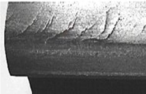
Figure 1
Photograph of surface cracks due to rolling contact fatigue - sometimes referred to as "gauge corner cracking" as this is where they usually occur.
Another of the reasons for slow inspection speeds using conventional NDT is the need for couplant between the transducer and the track using either liquid or dry couplant materials. EMATs have been used [2,3] or suggested 4 to measure both rail tracks and wheels by other workers and the use of non-contact ultrasonic measurements are still being investigated by a number of international research groups [5-8]. The real challenge and novelty with using EMATs to inspect the surface of the rail is the construction and design of a system that can actually work with sufficient signal:noise and an understanding of how to interpret the signal.
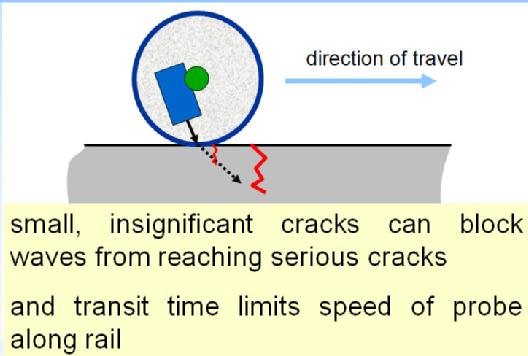
Figure 2
The schematic diagram above shows how the presence of a small defect can block the ultrasonic wave from travelling to the deeper defect, rendering it "invisible" to this type of measurement. One could of course angle waves to point forwards and backwards, but there is always a chance that smaller defects can lie either side of a deep defect.
Our approach to inspecting the rail head to detect and measure defect depth
Ultrasonic surface waves that are similar in behaviour to Rayleigh waves are an obvious candidate for surface breaking crack detection, or indeed for defects that lie just under the surface within the Rayleigh wave penetration depth 9-12. There are different approaches that may be used to detect a crack using a pitch-catch method. Strictly speaking, a Rayleigh wave only exists on a flat surface and as the surface of the rail head is curved the surface waves that propagate along or around the rail surface are a type of guided wave mode. Nevertheless these are still Rayleigh-like and for the purposes of this webpage we will refer to them as Rayleigh waves.
If a defect lies between the Rayleigh wave generator and detector then it will to some degree block the Rayleigh wave. The amplitude of a Rayleigh wave displacement decays with depth into the sample and most of the energy associated with a particular frequency lies within a depth equal to one wavelength at that frequency. Almost all of the energy lies within a depth corresponding to two wavelengths [9]. The different frequency components will effectively probe to different depths below the sample surface. In a measurement where we attempt to propagate a Rayleigh wave through a region containing a surface breaking crack, the crack depth can be estimated by the amount of Rayleigh wave energy or amplitude that is transmitted through or underneath that region. Closed or partially closed cracks can obviously complicate the analysis and increase the amount of Rayleigh wave energy transmitted through the crack compared to an open crack.
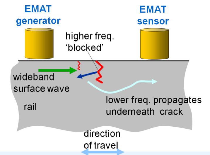
Figure 3
Schematic diagram showing how the EMATs were used in a pitch-catch type geometry for propagation of Rayleigh waves down the length of the rail head to measure and detect transverse cracks.
Results of crack depth measurements
The peak-to-peak amplitude is plotted in figure 4 as a function of slot depth. The cut-off frequency is estimated by comparison of the magnitude FFT of a defect free region with the region containing the slot. Cut-off frequency is plotted as a function of slot depth in the inset of figure 4. Both amplitude and frequency cut-off vary measurably for the slots in the depth range of 2.5 mm to 15 mm. By Using this type of approach we are able to not only detect the presence of a defect, but can also get a measurement of crack depth, which is crucial if the system is to be used in a practical application.
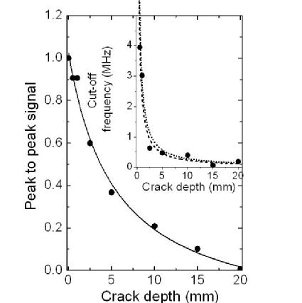
Figure 4
The plot above shows how the amplitude and frequency characteristics of the Rayleigh wave can be used to measure crack depth. This data was taken on a claibration block where crack depth is known.
One potential problem with EMATs is that their generation and detection efficiency is very stand-off dependent. We would hope to be able to maintain a fairly constant stand-off to overcome this issue, but obviously one needs to plan for the fact that this may not always be possible. This is where the frequency domain analysis comes into its own as the frequency content of the generated or detected wave characteristics hardly changes over a stand-off change of several millimetres. Thus, even though the amplitude of the detected wave may change because of the generator or detector EMAT changing stand-off through a "vibration" or "bounce", the relative frequency content on a defect free sample will remain constant.The variation of the frequency content (absolute and relative) is shown below in figure 5 with a change in stand-off between 1mm - 3.5mm, and in measuring defect depth, one looks at the relative change in frequency content.
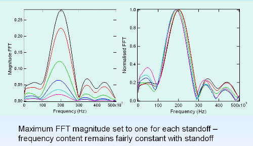
Figure 5
The plots above are the Fast Fourier Transforms of the detected surface wave taken at stand-offs between 3.5mm (lowest amplitude) to 1mm (highest amplitude. The graph on the left is the change in absolute frequency content, which is essentially a change in amplitude of the signal. The graph on the right shows the change in relative frequency content by normalising the Fast Fourier Transforms to have the same maximum amplitude - this is very small, but is predictable and is consistent with our numerical simulations.
Performing dynamic tests
We have conducted tests on both spinning rail rigs at high speeds and on track in-service at walking speeds. The tests from both of these are encouraging but have not been without some challenges. In the first tests on a 4m diameter rotating table, sections of curved tracks are bolted down to form a circle of rail track. The radius of curvature of this track is orders of magnitude sharper than would ever occur in reality and we have had to design a carriage system with independent suspension to deal with what are unrealistic issues in the rotating rail rig. Why do we need to do such tests? - Because it allows us to send the same known defects past the system many times to give us a good idea of accuracy and reliability. The picture below shows the set-up and by clicking the link you can see the video that was recorded for the first tests to check that the mechanics would hold the EMATs relaibly close to the rail. Note that this is a relatively large video file which could take some time to download.
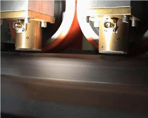
Figure 6
The photograph above shows some dynamic tests of the sensor delivery. Note that this test is less than 50mph and our target speed is 100mph. The EMATs in this photo are not connected, because as this was the first test, we did not want to attach cables to the EMATs just in case something happened that we hadn't allowed for.
Even thought these tests were conducted at half our target speed, one gets a good appreciation of the difficulties involved and how challenging these types of meaurements can be. The main issue with this test rig is the electromagnetic noise that the large electrical drive motors generate. Whilst this electrical noise is far higher than we would have in a real rail environment, there will still be some electrical noise and we have designed a system to deal with this which we will publish in due course.
The next stage of development
We have recently developed a novel EMAT transducer that has a low electrical noise susceptibility.
In Novenmber 2009 we reported a method that can be used to reduce the level of electromagentic inteerference on the acoustic signal from an EMAT. There are essentially two approaches:
1) Connect two EMATs in serial, one being counter-wound to the other and also being displaced from the other. Electromagnetic interference is picked up simultaneously on the two coils and as the coils are counterwoundm the net effect is that this noise signal at least partially cancels itself out. Whilst the acoutsic signal will be inverted, relative to each EMAT, they are also separated in time.
2) Two separate EMATs are used fairly close to each other and are connected to either a differential amplifier or two separate amplifiers. In the latter case, the data can be processed so as to mimimise the electrical noise picked uo by the EMAT by simply inverting one signal and adding it to the other. More sophisticated approaches can also be used to compensate for any difference in sensitivity of either the EMATs or preamplifiers.
In both of the above cases, the data can be improved by signal processing. Autocorrelation of the acoustic signals improves the signal:noise ratio and auto-correlation of the noise signals can be used as a step to removing the coincident noise from the total signal. The whole principle relies on the fact that the acoustic signals will arrive at significantly different times to each other, whilst the electrical noise pick up will be almost time coincident (and if not time coincident can be shifted slightly to obtain cancellation).
We have also developed a new EMAT design based detection approach, capable of measuring defect length and depth, and will also allow us to relibly detect shorted defects.
In order to undertake this next stage of research we are trying to secure research funding to properly the resource that is required.
Acknowledgements
Special thanks to Network Rail and Corus and colleagues at the Universities of Bristol and Birmingham who have supported and helped us with this research.
Thanks must also go to EPSRC for funding this project in the first instance.
References for further reading
[1]. Small J, Brook C, Ultrasonic instrumentation and transducers for rail inspection, Insight 44, pp373-374, 2002
[2]. Hirao, M; Ogi, H.; Fukuoka, H, Advanced Ultrasonic Method for Measuring Rail Axial Stresses with Electromagnetic Acoustic Transducer, Res. Nondest. Eval., 5, pp211-223, 1994
[3]. Rose JL, Avioli MJ, Mudge P, et al., Guided wave inspection potential of defects in rail NDT&E Int., 37, pp153-161, 2004
[4]. Armitage PR, The use of low-frequency Rayleigh waves to detect gauge corner cracking in railway lines, Insight, 44, pp369-372, 2002
[5]. Junger M, Thomas HM, Krull R, Eddy current test for operation-induced damaging on rails, Stahl Eisen, 119, pp107-110, 1999
[6]. di Scalea FL, McNamara J Ultrasonic NDE of railroad tracks: air-coupled cross-sectional inspection and long-range inspection, Insight, 45, pp394-401, 2003
[7]. Kenderian S, Cerniglia D, Djordjevic BB, et al., Rail track field testing using laser/air hybrid ultrasonic technique, Mater. Eval., 61, pp1129-1133, 2003
[8]. Pohl R et al , NDT techniques for railroad wheel and gauge corner inspection, NDT & E Int , 37 , pp 89-94 2004